آموزش کامل Excel 2007 - EN

[A M I R]

Lesson 2: Entering Excel Formulas and Formatting Data

​

[h=3]Perform Automatic Calculations
By default, Microsoft Excel recalculates the worksheet as you change cell entries. This

makes it easy for you to correct mistakes and analyze a variety of scenarios.

​

 

[A M I R]

Lesson 2: Entering Excel Formulas and Formatting Data

​

[h=4]EXERCISE 3

[h=4]Automatic Calculation

Make the changes described below and note how Microsoft Excel automatically recalculates

​

1. Move to cell A2.
2. Type 2.
3. Press the right arrow key. Excel changes the result in cell A4. Excel adds cell A2 to cell A3 and the new result appears in cell A4.
4. Move to cell B2.
5. Type 8.
6. Press the right arrow key. Excel subtracts cell B3 from cell B3 and the new result appears in cell B4.
7. Move to cell C2.
8. Type 4.
9. Press the right arrow key. Excel multiplies cell C2 by cell C3 and the new result appears in cell C4.
10. Move to cell D2.
11. Type 12.
12. Press the Enter key. Excel divides cell D2 by cell D3 and the new result appears in cell D4.

​

 

[A M I R]

Lesson 2: Entering Excel Formulas and Formatting Data


​

[h=3]Align Cell Entries

When you type text into a cell, by default your entry aligns with the left side of the cell. When you

type numbers into a cell, by default your entry aligns with the right side of the cell. You can change

the cell alignment. You can center, left-align, or right-align any cell entry. Look at cells A1 to D1. Note

that they are aligned with the left side of the cell.

​

​

 

[A M I R]

Lesson 2: Entering Excel Formulas and Formatting Data

​

[h=4]Center

To center cells A1 to D1:

1. Select cells A1 to D1.
2. Choose the Home tab.
3. Click the Center button
   
   in the Alignment group. Excel centers each cell's content.

​

 

[A M I R]

Lesson 2: Entering Excel Formulas and Formatting Data


​

[h=4]Left-Align

To left-align cells A1 to D1:

​

1. Select cells A1 to D1.
2. Choose the Home tab.
3. Click the Align Text Left
   
   button in the Alignment group. Excel left-aligns each cell's content.

​

 

[A M I R]

Lesson 2: Entering Excel Formulas and Formatting Data

​

[h=4]Right-Align
To right-align cells A1 to D1:

​

1. Select cells A1 to D1. Click in cell A1.
2. Choose the Home tab.
3. Click the Align Text Right
   
   button. Excel right-aligns the cell's content.
4. Click anywhere on your worksheet to clear the highlighting.

Note: You can also change the alignment of cells with numbers in them by using the alignment buttons.



​

 

[A M I R]

Lesson 2: Entering Excel Formulas and Formatting Data

​

[h=3]Perform Advanced Mathematical Calculations
When you perform mathematical calculations in Excel, be careful of precedence. Calculations

are performed from left to right, with multiplication and division performed before addition and subtraction.



​

 

[A M I R]

Lesson 2: Entering Excel Formulas and Formatting Data

​

[h=4]EXERCISE 4


[h=4]Advanced Calculations

1. Move to cell A7.
2. Type =3+3+12/2*4.
3. Press Enter.

Note: Microsoft Excel divides 12 by 2, multiplies the answer by 4, adds 3, and then adds another 3. The answer, 30, displays in cell A7.

​

To change the order of calculation, use parentheses. Microsoft Excel calculates the information in parentheses first.

1. Double-click in cell A7.
2. Edit the cell to read =(3+3+12)/2*4.
3. Press Enter.

Note: Microsoft Excel adds 3 plus 3 plus 12, divides the answer by 2, and then multiplies the result by 4. The answer, 36, displays in cell A7

​

​

 

[A M I R]

Lesson 2: Entering Excel Formulas and Formatting Data

​

[h=3]Copy, Cut, Paste, and Cell Addressing
In Excel, you can copy data from one area of a worksheet and place the data you copied

anywhere in the same or another worksheet. In other words, after you type information into

a worksheet, if you want to place the same information somewhere else, you do not have to

retype the information. You simple copy it and then paste it in the new location.


You can use Excel's Cut feature to remove information from a worksheet. Then you

can use the Paste feature to place the information you cut anywhere in the same or another

worksheet. In other words, you can move information from one place in a worksheet to

another place in the same or different worksheet by using the Cut and Paste features.


Microsoft Excel records cell addresses in formulas in three different ways, called absolute, relative, and mixed. The way

a formula is recorded is important when you copy it. With relative cell addressing, when you copy a formula from

one area of the worksheet to another, Excel records the position of the cell relative to the cell that originally

contained the formula. With absolute cell addressing, when you copy a formula from one area of the worksheet

to another, Excel references the same cells, no matter where you copy the formula. You can use mixed cell

addressing to keep the row constant while the column changes, or vice versa. The following exercises demonstrate.





​

 

[A M I R]

Lesson 2: Entering Excel Formulas and Formatting Data

​

[h=4]EXERCISE 5


[h=4]Copy, Cut, Paste, and Cell Addressing

1. Move to cell A9.
2. Type 1. Press Enter. Excel moves down one cell.
3. Type 1. Press Enter. Excel moves down one cell.
4. Type 1. Press Enter. Excel moves down one cell.
5. Move to cell B9.
6. Type 2. Press Enter. Excel moves down one cell.
7. Type 2. Press Enter. Excel moves down one cell.
8. Type 2. Press Enter. Excel moves down one cell.

In addition to typing a formula as you did in Lesson 1, you can also enter formulas by using Point mode. When

you are in Point mode, you can enter a formula either by clicking on a cell or by using the arrow keys.

1. Move to cell A12.
2. Type =.
3. Use the up arrow key to move to cell A9.
4. Type +.
5. Use the up arrow key to move to cell A10.
6. Type +.
7. Use the up arrow key to move to cell A11.
8. Click the check mark on the Formula bar. Look at the Formula bar. Note that the formula you entered is displayed there.

​

​

 

[A M I R]

Lesson 2: Entering Excel Formulas and Formatting Data

​

[h=4]Copy with the Ribbon
To copy the formula you just entered, follow these steps:

​

1. You should be in cell A12.
2. Choose the Home tab.
3. Click the Copy
   
   button in the Clipboard group. Excel copies the formula in cell A12.

​

1. Press the right arrow key once to move to cell B12.
2. Click the Paste
   
   button in the Clipboard group. Excel pastes the formula in cell A12 into cell B12.
3. Press the Esc key to exit the Copy mode.

Compare the formula in cell A12 with the formula in cell B12 (while in the respective cell, look at

the Formula bar). The formulas are the same except that the formula in cell A12 sums the entries

in column A and the formula in cell B12 sums the entries in column B. The formula was copied in a relative fashion.


Before proceeding with the next part of the exercise, you must copy the information in

cells A7 to B9 to cells C7 to D9. This time you will copy by using the Mini toolbar.


​

 

[A M I R]

Lesson 2: Entering Excel Formulas and Formatting Data

​

[h=4]Copy with the Mini Toolbar

​

1. Select cells A9 to B11. Move to cell A9. Press the Shift key. While holding down the Shift key, press the down arrow key twice. Press the right arrow key once. Excel highlights A9 to B11.
2. Right-click. A context menu and a Mini toolbar appear.
3. Click Copy, which is located on the context menu. Excel copies the information in cells A9 to B11.

​

1. Move to cell C9.
2. Right-click. A context menu appears.
3. Click Paste. Excel copies the contents of cells A9 to B11 to cells C9 to C11.

​

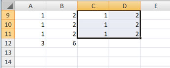
1. Press Esc to exit Copy mode.

​

 

[A M I R]

Lesson 2: Entering Excel Formulas and Formatting Data

​

[h=4]Absolute Cell Addressing
You make a cell address an absolute cell address by placing a dollar sign in front of the row

and column identifiers. You can do this automatically by using the F4 key. To illustrate:

1. Move to cell C12.
2. Type =.
3. Click cell C9.
4. Press F4. Dollar signs appear before the C and the 9.
5. Type +.
6. Click cell C10.
7. Press F4. Dollar signs appear before the C and the 10.
8. Type +.
9. Click cell C11.
10. Press F4. Dollar signs appear before the C and the 11.
11. Click the check mark on the formula bar. Excel records the formula in cell C12.

​

​

 

[A M I R]

Lesson 2: Entering Excel Formulas and Formatting Data

​

[h=4]Copy and Paste with Keyboard Shortcuts
Keyboard shortcuts are key combinations that enable you to perform tasks by using the

keyboard. Generally, you press and hold down a key while pressing a letter. For example, Ctrl+c means

you should press and hold down the Ctrl key while pressing "c." This tutorial notates key combinations as follows:

Press Ctrl+c.
​

Now copy the formula from C12 to D12. This time, copy by using keyboard shortcuts.

1. Move to cell C12.
2. Hold down the Ctrl key while you press "c" (Ctrl+c). Excel copies the contents of cell C12.
3. Press the right arrow once. Excel moves to D12.
4. Hold down the Ctrl key while you press "v" (Ctrl+v). Excel pastes the contents of cell C12 into cell D12.
5. Press Esc to exit the Copy mode.

​

Compare the formula in cell C12 with the formula in cell D12 (while in the respective cell, look

at the Formula bar). The formulas are exactly the same. Excel copied the formula from cell

C12 to cell D12. Excel copied the formula in an absolute fashion. Both formulas sum column C.


​

 

[A M I R]

Lesson 2: Entering Excel Formulas and Formatting Data

​

[h=4]Mixed Cell Addressing
You use mixed cell addressing to reference a cell when you want to copy part of it absolute and part relative. For

example, the row can be absolute and the column relative. You can use the F4 key to create a mixed cell reference.

1. Move to cell E1.
2. Type =.
3. Press the up arrow key once.
4. Press F4.
5. Press F4 again. Note that the column is relative and the row is absolute.
6. Press F4 again. Note that the column is absolute and the row is relative.
7. Press Esc.

​

 

[A M I R]

Lesson 2: Entering Excel Formulas and Formatting Data

​

[h=4]Cut and Paste

You can move data from one area of a worksheet to another.

​

1. Select cells D9 to D12
2. Choose the Home tab.
3. Click the Cut
   
   button.
4. Move to cell G1.

1. Click the Paste button
   
   . Excel moves the contents of cells D9 to D12 to cells G1 to G4.

The keyboard shortcut for Cut is Ctrl+x. The steps for cutting and pasting with a keyboard shortcut are:

1. Select the cells you want to cut and paste.
2. Press Ctrl+x.
3. Move to the upper-left corner of the block of cells into which you want to paste.
4. Press Ctrl+v. Excel cuts and pastes the cells you selected.

​

 

[A M I R]

Lesson 2: Entering Excel Formulas and Formatting Data



[h=3]

Insert and Delete Columns and Rows

You can insert and delete columns and rows. When you delete a column, you delete everything in the

column from the top of the worksheet to the bottom of the worksheet. When you delete a row, you

delete the entire row from left to right. Inserting a column or row inserts a completely new column or row.


​

​

 

[A M I R]

Lesson 2: Entering Excel Formulas and Formatting Data

​

[h=4]EXERCISE 6



[h=4]Insert and Delete Columns and Rows

To delete columns F and G:

​

1. Click the column F indicator and drag to column G.
2. Click the down arrow next to Delete in the Cells group. A menu appears.
3. Click Delete Sheet Columns. Excel deletes the columns you selected.
4. Click anywhere on the worksheet to remove your selection.

To delete rows 7 through 12:

​

1. Click the row 7 indicator and drag to row 12.
2. Click the down arrow next to Delete in the Cells group. A menu appears.
3. Click Delete Sheet Rows. Excel deletes the rows you selected.
4. Click anywhere on the worksheet to remove your selection.

To insert a column:

1. Click on A to select column A.
2. Click the down arrow next to Insert in the Cells group. A menu appears.
3. Click Insert Sheet Columns. Excel inserts a new column.
4. Click anywhere on the worksheet to remove your selection.

To insert rows:

1. Click on 1 and then drag down to 2 to select rows 1 and 2.
2. Click the down arrow next to Insert in the Cells group. A menu appears.
3. Click Insert Sheet Rows. Excel inserts two new rows.
4. Click anywhere on the worksheet to remove your selection.

Your worksheet should look like the one shown here.

​

​

 

[A M I R]

Lesson 2: Entering Excel Formulas and Formatting Data

​

[h=3]Create Borders

You can use borders to make entries in your Excel worksheet stand out. You can choose from several types of

borders. When you press the down arrow next to the Border button

, a menu appears. By making the

proper selection from the menu, you can place a border on the top, bottom, left, or right side of the selected

cells; on all sides; or around the outside border. You can have a thick outside border or a border with a

single-line top and a double-line bottom. Accountants usually place a single underline above a final number

and a double underline below. The following illustrates:



​

 

[A M I R]

Lesson 2: Entering Excel Formulas and Formatting Data

​

[h=4]EXERCISE 7


[h=4]Create Borders

1. Select cells B6 to E6.

​

1. Choose the Home tab.
2. Click the down arrow next to the Borders button
   
   . A menu appears.
3. Click Top and Double Bottom Border. Excel adds the border you chose to the selected cells.

​

​