آموزش کامل Excel 2007 - EN

[A M I R]

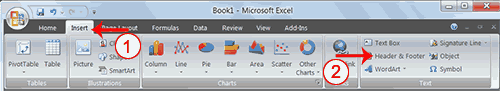
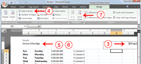
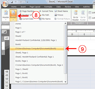
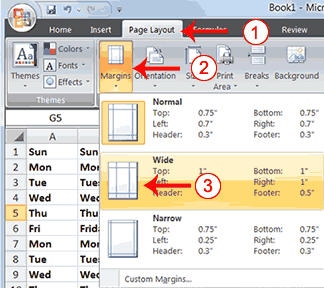
Lesson 3: Creating Excel Functions, Filling Cells, and Printing


​

[h=3]Understanding Functions
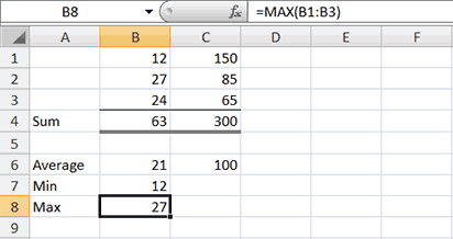
Functions are prewritten formulas. Functions differ from regular formulas in that you supply

the value but not the operators, such as +, -, *, or /. For example, you can use the SUM

function to add. When using a function, remember the following:

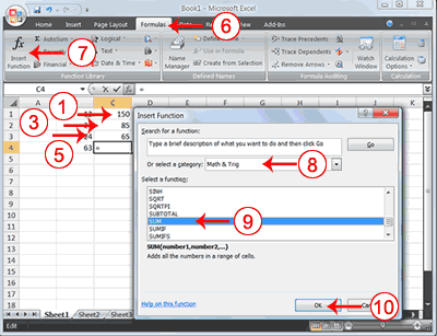
Use an equal sign to begin a formula.

Specify the function name.
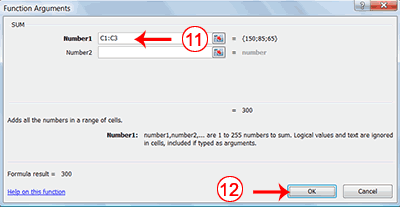
Enclose arguments within parentheses. Arguments are values on which you want to perform the calculation. For example, arguments specify the numbers or cells you want to add.
Use a comma to separate arguments.
​

Here is an example of a function:

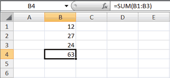
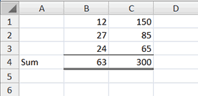
=SUM(2,13,A1,B2:C7)
​

In this function:

The equal sign begins the function.
SUM is the name of the function.
2, 13, A1, and B2:C7 are the arguments.
Parentheses enclose the arguments.
Commas separate the arguments.
​

After you type the first letter of a function name, the AutoComplete list appears. You can double-click

on an item in the AutoComplete list to complete your entry quickly. Excel will complete the function

name and enter the first parenthesis.



​

 

[A M I R]

Lesson 3: Creating Excel Functions, Filling Cells, and Printing

​

[h=4]EXERCISE 1



[h=4]Functions


The SUM function adds argument values.

​

1. Open Microsoft Excel.
2. Type 12 in cell B1.
3. Press Enter.
4. Type 27 in cell B2.
5. Press Enter.
6. Type 24 in cell B3.
7. Press Enter.
8. Type =SUM(B1:B3) in cell A4.
9. Press Enter. The sum of cells B1 to B3, which is 63, appears.

​

 

[A M I R]

Lesson 3: Creating Excel Functions, Filling Cells, and Printing

​

[h=4]Alternate Method: Enter a Function with the Ribbon

​

1. Type 150 in cell C1.
2. Press Enter.
3. Type 85 in cell C2.
4. Press Enter.
5. Type 65 in cell C3.
6. Choose the Formulas tab.
7. Click the Insert Function button. The Insert Function dialog box appears.
8. Choose Math & Trig in the Or Select A Category box.
9. Click Sum in the Select A Function box.
10. Click OK. The Function Arguments dialog box appears.

​

1. Type C1:C3 in the Number1 field, if it does not automatically appear.
2. Click OK. The sum of cells C1 to C3, which is 300, appears.

​

 

[A M I R]

Lesson 3: Creating Excel Functions, Filling Cells, and Printing

​

[h=4]Format worksheet

1. Move to cell A4.
2. Type the word Sum.
3. Select cells B4 to C4.
4. Choose the Home tab.
5. Click the down arrow next to the Borders button
   
   .
6. Click Top and Double Bottom Border.

As you learned in Lesson 2, you can also calculate a sum by using the AutoSum button

.



​

 

[A M I R]

Lesson 3: Creating Excel Functions, Filling Cells, and Printing

​

[h=4]Calculate an Average




You can use the AVERAGE function to calculate the average of a series of numbers.

​

1. Move to cell A6.
2. Type Average. Press the right arrow key to move to cell B6.
3. Type =AVERAGE(B1:B3).
4. Press Enter. The average of cells B1 to B3, which is 21, appears.

​

 

[A M I R]

Lesson 3: Creating Excel Functions, Filling Cells, and Printing

​

[h=4]Calculate an Average with the AutoSum Button

In Microsoft Excel, you can use the AutoSum button

to calculate an average.

1. Move to cell C6.
2. Choose the Home tab.
3. Click the down arrow next to the AutoSum button
   
   .
4. Click Average.

​

1. Select cells C1 to C3.
2. Press Enter. The average of cells C1 to C3, which is 100, appears.

​

 

[A M I R]

Lesson 3: Creating Excel Functions, Filling Cells, and Printing

​

[h=4]Find the Lowest Number


You can use the MIN function to find the lowest number in a series of numbers.

​

1. Move to cell A7.
2. Type Min.
3. Press the right arrow key to move to cell B7.
4. Type = MIN(B1:B3).
5. Press Enter. The lowest number in the series, which is 12, appears.

Note: You can also use the drop-down button next to the AutoSum button

to calculate minimums, maximums, and counts.



​

 

[A M I R]

Lesson 3: Creating Excel Functions, Filling Cells, and Printing

​

[h=4]Find the Highest Number



You can use the MAX function to find the highest number in a series of numbers.

.

​

1. Move to cell A8.
2. Type Max.
3. Press the right arrow key to move to cell B8.
4. Type = MAX(B1:B3).
5. Press Enter. The highest number in the series, which is 27, appears.

​

 

[A M I R]

[h=4]Count the Numbers in a Series of Numbers

You can use the count function to count the number of numbers in a series.

1. Move to cell A9.
2. Type Count.
3. Press the right arrow key to move to cell B9.
4. Choose the Home tab.
5. Click the down arrow next to the AutoSum button
   
   .
6. Click Count Numbers. Excel places the count function in cell C9 and takes a guess at which cells you want to count. The guess is incorrect, so you must select the proper cells.

​

1. Select B1 to B3.
2. Press Enter. The number of items in the series, which is 3, appears.

​

 

[A M I R]

Lesson 3: Creating Excel Functions, Filling Cells, and Printing

​

[h=3]Fill Cells Automatically



You can use Microsoft Excel to fill cells automatically with a series. For example, you can have Excel

automatically fill your worksheet with days of the week, months of the year, years, or other types of series.

​

 

[A M I R]

Lesson 3: Creating Excel Functions, Filling Cells, and Printing

​

[h=4]EXERCISE 2

[h=4]Fill Cells Automatically

The following demonstrates filling the days of the week
:

1. Click the Sheet2 tab. Excel moves to Sheet2.
2. Move to cell A1.
3. Type Sun.
4. Move to cell B1.
5. Type Sunday.
6. Select cells A1 to B1.
7. Choose the Home tab.
8. Click the Bold button
   
   . Excel bolds cells A1 to B1.
9. Find the small black square in the lower-right corner of the selected area. The small black square is called the fill handle.
10. Grab the fill handle and drag with your mouse to fill cells A1 to B14. Note how the days of the week fill the cells in a series. Also, note that the Auto Fill Options button appears.

​

[h=4]Copy Cells

​

1. Click the Auto Fill Options button. The Auto Fill Options menu appears.
2. Choose the Copy Cells radio button. The entry in cells A1 and B1 are copied to all the highlighted cells.
3. Click the Auto Fill Options button again.
4. Choose the Fill Series radio button. The cells fill as a series from Sunday to Saturday again.
5. Click the Auto Fill Options button again.
6. Choose the Fill Without Formatting radio button. The cells fill as a series from Sunday to Saturday, but the entries are not bolded.
7. Click the Auto Fill Options button again.
8. Choose the Fill Weekdays radio button. The cells fill as a series from Monday to Friday.

​

 

[A M I R]

Lesson 3: Creating Excel Functions, Filling Cells, and Printing

​

[h=4]Adjust Column Width

Some of the entries in column B are too long to fit in the column. You can quickly adjust the column width to fit the longest entry.

1. Move your mouse pointer over the line that separates column B and C. The Width Indicator appears.

1. Double-click. The Column adjusts to fit the longest entry.

After you complete the remainder of the exercise, your worksheet will look like the one shown here.

​

​

 

[A M I R]

Lesson 3: Creating Excel Functions, Filling Cells, and Printing

​

[h=4]Fill Times

The following demonstrates filling time:

1. Type 1:00 into cell C1.
2. Grab the fill handle and drag with your mouse to highlight cells C1 to C14. Note that each cell fills, using military time.
3. Press Esc and then click anywhere on the worksheet to remove the highlighting.

To change the format of the time:

1. Select cells C1 to C14.
2. Choose the Home tab.
3. Click the down arrow next to the number format box
   
   . A menu appears.
4. Click Time. Excel changes the format of the time.

​

 

[A M I R]

Lesson 3: Creating Excel Functions, Filling Cells, and Printing

​

[h=4]Fill Numbers

You can also fill numbers.

Type a 1 in cell D1.

1. Grab the fill handle and drag with your mouse to highlight cells D1 to D14. The number 1 fills each cell.
2. Click the Auto Fill Options button.
3. Choose the Fill Series radio button. The cells fill as a series, starting with 1, 2, 3.

Here is another interesting fill feature.

1. Go to cell E1.
2. Type Lesson 1.
3. Grab the fill handle and drag with your mouse to highlight cells E1 to E14. The cells fill in as a series: Lesson 1, Lesson 2, Lesson 3, and so on.

​

 

[A M I R]

Lesson 3: Creating Excel Functions, Filling Cells, and Printing

​

[h=3]Create Headers and Footers

You can use the Header & Footer button on the Insert tab to create headers and footers. A header

is text that appears at the top of every page of your printed worksheet. A footer is text that appears

at the bottom of every page of your printed worksheet. When you click the Header & Footer

button, the Design context tab appears and Excel changes to Page Layout view. A context tab

is a tab that only appears when you need it. Page Layout view structures your worksheet so

that you can easily change the format of your document. You usually work in Normal view.



You can type in your header or footer or you can use predefined headers and footers. To find

predefined headers and footers, click the Header or Footer button or use the Header & Footer

Elements group's buttons. When you choose a header or footer by clicking the Header or Footer

button, Excel centers your choice. The table shown here describes each of the Header & Footer

Elements group button options.

Header & Footer Elements​
Button	Purpose
Page Number	Inserts the page number.
Number of Pages	Inserts the number of pages in the document.
Current Time	Inserts the current time.
File Path	Inserts the path to the document.
File Name	Inserts the file name.
Sheet Name	Inserts the name of the worksheet.
Picture	Enables you to insert a picture.

Both the header and footer areas are divided into three sections: left, right, and center. When you choose

a Header or Footer from the Header & Footer Elements group, where you place your information determines

whether it appears on the left, right, or center of the printed page. You use the Go To Header and Go To

Footer buttons on the Design tab to move between the header and footer areas of your worksheet.
​

 

[A M I R]

Lesson 3: Creating Excel Functions, Filling Cells, and Printing



[h=4]EXERCISE 3

[h=4]Insert Headers and Footers

​

1. Choose the Insert tab.
2. Click the Header & Footer button in the Text group. Your worksheet changes to Page Layout view and the Design context tab appears. Note that your cursor is located in the center section of the header area.

​

1. Click the right side of the header area.
2. Click Page Number in the Header & Footer Elements group. When you print your document, Excel will place the page number in the upper-right corner.
3. Click the left side of the Header area.
4. Type your name. When you print your document, Excel will place your name in the upper-left corner.
5. Click the Go To Footer button. Excel moves to the footer area.

​

1. Click the Footer button. A menu appears.
2. Click the path to your document. Excel will place the path to your document at the bottom of every printed page.

​

​

 

[A M I R]

Lesson 3: Creating Excel Functions, Filling Cells, and Printing

​

[h=4]Return to Normal View
To return to Normal view:

1. Choose the View tab.
2. Click the Normal button in the Workbook Views group.

​

 

[A M I R]

Lesson 3: Creating Excel Functions, Filling Cells, and Printing

​

[h=3]Set Print Options

There are many print options. You set print options on the Page Layout tab. Among other

things, you can set your margins, set your page orientation, and select your paper size.


Margins define the amount of white space that appears on the top, bottom, left, and right edges

of your document. The Margin option on the Page Layout tab provides several standard margin sizes from which you can choose
.

There are two page orientations: portrait and landscape. Paper, such as paper sized 8 1/2 by 11, is longer

on one edge than it is on the other. If you print in Portrait, the shortest edge of the paper becomes the top

of the page. Portrait is the default option. If you print in Landscape, the longest edge of the paper becomes the top of the page.

Portrait​

Landscape ​

Paper comes in a variety of sizes. Most business correspondence uses 8 1/2 by 11 paper, which

is the default page size in Excel. If you are not using 8 1/2 by 11 paper, you can use the Size

option on the Page Layout tab to change the Size setting.


​

 

[A M I R]

Lesson 3: Creating Excel Functions, Filling Cells, and Printing

​

[h=4]EXERCISE 4

[h=4]Set the Page Layout

​

1. Choose the Page Layout tab.
2. Click Margins in the Page Setup group. A menu appears.
3. Click Wide. Word sets your margins to the Wide settings.

[h=4]Set the Page Orientation

​

1. Choose the Page Layout tab.
2. Click Orientation in the Page Setup group. A menu appears.
3. Click Landscape. Excel sets your page orientation to landscape.

[h=4]Set the Paper Size

​

1. Choose the Page Layout tab.
2. Click Size in the Page Setup group. A menu appears.
3. Click the paper size you are using. Excel sets your page size.

​

 

[A M I R]

Lesson 3: Creating Excel Functions, Filling Cells, and Printing

​

[h=3]Print


The simplest way to print is to click the Office button, highlight Print on the menu that appears, and

then click Quick Print in the Preview and Print the Document pane. Dotted lines appear on your

screen, and your document prints. The dotted lines indicate the right, left, top, and bottom edges of your printed pages.


You can also use the Print Preview option to print. When using Print Preview, you can see

onscreen how your printed document will look when you print it. If you click the Page Setup

button while in Print Preview mode, you can set page settings such as centering your data on the page.


If your document is several pages long, you can use the Next Page and Previous Page buttons

to move forward and backward through your document. If you check the Show Margins check

box, you will see margin lines on your document. You can click and drag the margin markers

to increase or decrease the size of your margins. To return to Excel, click the Close Print

Preview button.


You click the Print button when you are ready to print. The Print dialog box appears. You can

choose to print the entire worksheet or specific pages. If you want to print specific pages, enter

the page numbers in the From and To fields. You can enter the number of copies you want to

print in the Number of Copies field.



​