آموزش کامل Excel 2007 - EN

[A M I R]

Lesson 2: Entering Excel Formulas and Formatting Data

​

[h=3]Merge and Center

Sometimes, particularly when you give a title to a section of your worksheet, you will want

to center a piece of text over several columns or rows. The following example shows you how.



​

 

[A M I R]

Lesson 2: Entering Excel Formulas and Formatting Data

​

[h=4]EXERCISE 8

[h=4]Merge and Center

​

1. Go to cell B2.
2. Type Sample Worksheet.
3. Click the check mark on the Formula bar.
4. Select cells B2 to E2.
5. Choose the Home tab.
6. Click the Merge and Center button
   
   in the Alignment group. Excel merges cells B2, C2, D2, and E2 and then centers the content.

​

Note: To unmerge cells:

1. Select the cell you want to unmerge.
2. Choose the Home tab.
3. Click the down arrow next to the Merge and Center button.
   
   A menu appears.
4. Click Unmerge Cells. Excel unmerges the cells.

​

 

[A M I R]

Lesson 2: Entering Excel Formulas and Formatting Data


​

[h=3]Add Background Color
To make a section of your worksheet stand out, you can

add background color to a cell or group of cells.






​

 

[A M I R]

Lesson 2: Entering Excel Formulas and Formatting Data

​

[h=4]EXERCISE 9

[h=4]Add Background Color

1. Select cells B2 to E3.

1. Choose the Home tab.
2. Click the down arrow next to the Fill Color button
   
   .
3. Click the color dark blue. Excel places a dark blue background in the cells you selected.

​

​

 

[A M I R]

Lesson 2: Entering Excel Formulas and Formatting Data

​

[h=3]Change the Font, Font Size, and Font Color



A font is a set of characters represented in a single typeface. Each character within a font is created

by using the same basic style. Excel provides many different fonts from which you can choose. The

size of a font is measured in points. There are 72 points to an inch. The number of points assigned

to a font is based on the distance from the top to the bottom of its longest character. You can change

the Font, Font Size, and Font Color of the data you enter into Excel.



​

 

[A M I R]

Lesson 2: Entering Excel Formulas and Formatting Data

​

[h=4]EXERCISE 10


[h=4]Change the Font

1. Select cells B2 to E3.

​

1. Choose the Home tab.
2. Click the down arrow next to the Font box. A list of fonts appears. As you scroll down the list of fonts, Excel provides a preview of the font in the cell you selected.
3. Find and click Times New Roman in the Font box. Note: If Times New Roman is your default font, click another font. Excel changes the font in the selected cells.

[h=4]Change the Font Size

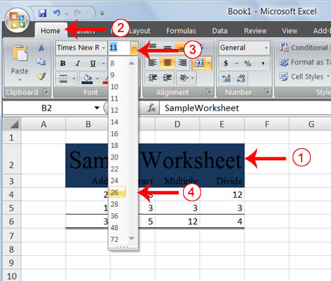
1. Select cell B2.
2. Choose the Home tab.
3. Click the down arrow next to the Font Size box. A list of font sizes appears. As you scroll up or down the list of font sizes, Excel provides a preview of the font size in the cell you selected.
4. Click 26. Excel changes the font size in cell B2 to 26.

[h=4]Change the Font Color

​

1. Select cells B2 to E3.
2. Choose the Home tab.
3. Click the down arrow next to the Font Color button
   
   .
4. Click on the color white. Your font color changes to white.

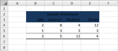
Your worksheet should look like the one shown here.

​

​

 

[A M I R]

Lesson 2: Entering Excel Formulas and Formatting Data

​

[h=3]Move to a New Worksheet

In Microsoft Excel, each workbook is made up of several worksheets. Each worksheet has a tab. By

default, a workbook has three sheets and they are named sequentially, starting with Sheet1. The

name of the worksheet appears on the tab. Before moving to the next topic, move to a new

worksheet. The exercise that follows shows you how.

​

 

[A M I R]

Lesson 2: Entering Excel Formulas and Formatting Data

​

[h=4]EXERCISE 11


[h=4]Move to a New Worksheet

• Click Sheet2 in the lower-left corner of the screen. Excel moves to Sheet2.

​

​

 

[A M I R]

Lesson 2: Entering Excel Formulas and Formatting Data

​

[h=3]Bold, Italicize, and Underline

When creating an Excel worksheet, you may want to emphasize the contents of cells by

bolding, italicizing, and/or underlining. You can easily bold, italicize, or underline text with

Microsoft Excel. You can also combine these features—in other words, you

can bold, italicize, and underline a single piece of text.



In the exercises that follow, you will learn different methods you can use to bold, italicize, and underline.



​

 

[A M I R]

Lesson 2: Entering Excel Formulas and Formatting Data




​

[h=4]EXERCISE 12


[h=4]Bold with the Ribbon
[h=4]Bold with the Ribbon [h=4]

1. Type Bold in cell A1.
2. Click the check mark located on the Formula bar.
3. Choose the Home tab.
4. Click the Bold button
   
   . Excel bolds the contents of the cell.
5. Click the Bold button
   
   again if you wish to remove the bold.

[h=4]Italicize with the Ribbon

1. Type Italic in cell B1.
2. Click the check mark located on the Formula bar.
3. Choose the Home tab.
4. Click the Italic button
   
   . Excel italicizes the contents of the cell.
5. Click the Italic button
   
   again if you wish to remove the italic.

[h=4]Underline with the Ribbon Microsoft Excel provides two types of underlines. The exercises that follow illustrate them.
Single Underline:

1. Type Underline in cell C1.
2. Click the check mark located on the Formula bar.
3. Choose the Home tab.
4. Click the Underline button
   
   . Excel underlines the contents of the cell.
5. Click the Underline button
   
   again if you wish to remove the underline.

[h=4]Double Underline

1. Type Underline in cell D1.
2. Click the check mark located on the Formula bar.
3. Choose the Home tab.
4. Click the down arrow next to the Underline button
   
   and then click Double Underline. Excel double-underlines the contents of the cell. Note that the Underline button changes to the button shown here
   
   , a D with a double underline under it. Then next time you click the Underline button, you will get a double underline. If you want a single underline, click the down arrow next to the Double Underline button
   
   and then choose Underline.
5. Click the double underline button again if you wish to remove the double underline.

[h=4]Bold, Underline, and Italicize

1. Type All three in cell E1.
2. Click the check mark located on the Formula bar.
3. Choose the Home tab.
4. Click the Bold button
   
   . Excel bolds the cell contents.
5. Click the Italic button
   
   . Excel italicizes the cell contents.
6. Click the Underline button
   
   . Excel underlines the cell contents.

​

 

[A M I R]

Lesson 2: Entering Excel Formulas and Formatting Data

​

Alternate Method: Bold with Shortcut Keys

1. Type Bold in cell A2.
2. Click the check mark located on the Formula bar.
3. Hold down the Ctrl key while pressing "b" (Ctrl+b). Excel bolds the contents of the cell.
4. Press Ctrl+b again if you wish to remove the bolding.

[h=4]Alternate Method: Italicize with Shortcut Keys

1. Type Italic in cell B2. Note: Because you previously entered the word Italic in column B, Excel may enter the word in the cell automatically after you type the letter I. Excel does this to speed up your data entry.
2. Click the check mark located on the Formula bar.
3. Hold down the Ctrl key while pressing "i" (Ctrl+i). Excel italicizes the contents of the cell.
4. Press Ctrl+i again if you wish to remove the italic formatting.

[h=4]Alternate Method: Underline with Shortcut Keys

1. Type Underline in cell C2.
2. Click the check mark located on the Formula bar.
3. Hold down the Ctrl key while pressing "u" (Ctrl+u). Excel applies a single underline to the cell contents.
4. Press Ctrl+u again if you wish to remove the underline.

[h=4]Bold, Italicize, and Underline with Shortcut Keys

1. Type All three in cell D2.
2. Click the check mark located on the Formula bar.
3. Hold down the Ctrl key while pressing "b" (Ctrl+b). Excel bolds the cell contents.
4. Hold down the Ctrl key while pressing "i" (Ctrl+i). Excel italicizes the cell contents.
5. Hold down the Ctrl key while pressing "u" (Ctrl+u). Excel applies a single underline to the cell contents.

​

 

[A M I R]

Lesson 2: Entering Excel Formulas and Formatting Data

​

[h=3]Work with Long Text




Whenever you type text that is too long to fit into a cell, Microsoft Excel attempts to display

all the text. It left-aligns the text regardless of the alignment you have assigned to it, and it

borrows space from the blank cells to the right. However, a long text entry will never write

over cells that already contain entries—instead, the cells that contain entries cut off the

long text. The following exercise illustrates this.



​

 

[A M I R]

Lesson 2: Entering Excel Formulas and Formatting Data

​

[h=4]EXERCISE 13


[h=4]Work with Long Text

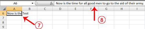
1. Move to cell A6.
2. Type Now is the time for all good men to go to the aid of their army.
3. Press Enter. Everything that does not fit into cell A6 spills over into the adjacent cell.

​

1. Move to cell B6.
2. Type Test.
3. Press Enter. Excel cuts off the entry in cell A6.

​

1. Move to cell A6.
2. Look at the Formula bar. The text is still in the cell.

​

 

[A M I R]

Lesson 2: Entering Excel Formulas and Formatting Data

​

[h=3]Change A Column's Width

You can increase column widths. Increasing the column width enables you to see the long text.



​

 

[A M I R]

Lesson 2: Entering Excel Formulas and Formatting Data

​

[h=4]EXERCISE 14


[h=4]Change Column Width

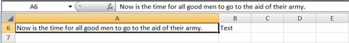
1. Make sure you are in any cell under column A.
2. Choose the Home tab.
3. Click the down arrow next to Format in the Cells group.
4. Click Column Width. The Column Width dialog box appears.
5. Type 55 in the Column Width field.
6. Click OK. Column A is set to a width of 55. You should now be able to see all of the text.

[h=4]Change a Column Width by Dragging You can also change the column width with the cursor.

1. Place the mouse pointer on the line between the B and C column headings. The mouse pointer should look like the one displayed here
   
   , with two arrows.
2. Move your mouse to the right while holding down the left mouse button. The width indicator
   
   appears on the screen.
3. Release the left mouse button when the width indicator shows approximately 20. Excel increases the column width to 20.

​

 

[A M I R]

Lesson 2: Entering Excel Formulas and Formatting Data

​

[h=3]Format Numbers

You can format the numbers you enter into Microsoft Excel. For example, you can add

commas to separate thousands, specify the number of decimal places, place a dollar

sign in front of a number, or display a number as a percent.

​

 

[A M I R]

Lesson 2: Entering Excel Formulas and Formatting Data

​

[h=4]EXERCISE 15


[h=4]Format Numbers

1. Move to cell B8.
2. Type 1234567.
3. Click the check mark on the Formula bar.

​

1. Choose the Home tab.
2. Click the down arrow next to the Number Format box. A menu appears.
3. Click Number. Excel adds two decimal places to the number you typed.

1. Click the Comma Style button
   
   . Excel separates thousands with a comma.
2. Click the Accounting Number Format button
   
   . Excel adds a dollar sign to your number.
3. Click twice on the Increase Decimal button
   
   to change the number format to four decimal places.
4. Click the Decrease Decimal button
   
   if you wish to decrease the number of decimal places.

[h=4]Change a decimal to a percent.

​

1. Move to cell B9.
2. Type .35 (note the decimal point).
3. Click the check mark on the formula bar.

​

1. Choose the Home tab.
2. Click the Percent Style button
   
   . Excel turns the decimal to a percent.

This is the end of Lesson 2. You can save and close your file. See Lesson 1 to learn how to save and close a file.
​

​

 

[A M I R]

[h=2]Lesson 3: Creating Excel Functions, Filling Cells, and Printing

By using functions, you can quickly and easily make many useful calculations, such as finding an


average, the highest number, the lowest number, and a count of the number of items in a

list. Microsoft Excel has many functions that you can use.
​

 

[A M I R]

Lesson 3: Creating Excel Functions, Filling Cells, and Printing

​

[h=3]Using Reference Operators

To use functions, you need to understand reference operators. Reference operators refer to a

cell or a group of cells. There are two types of reference operators: range and union.


A range reference refers to all the cells between and including the reference. A range

reference consists of two cell addresses separated by a colon. The reference A1:A3 includes

cells A1, A2, and A3. The reference A1:C3 includes cells A1, A2, A3, B1, B2, B3, C1, C2, and C3.


A union reference includes two or more references. A union reference consists of two or more

numbers, range references, or cell addresses separated by a comma. The

reference A7,B8:B10,C9,10 refers to cells A7, B8 to B10, C9 and the number 10.
​

 

[A M I R]

Lesson 3: Creating Excel Functions, Filling Cells, and Printing

​

[h=3]Using Reference Operators

To use functions, you need to understand reference operators. Reference operators refer to a

cell or a group of cells. There are two types of reference operators: range and union.


A range reference refers to all the cells between and including the reference. A range

reference consists of two cell addresses separated by a colon. The reference A1:A3 includes

cells A1, A2, and A3. The reference A1:C3 includes cells A1, A2, A3, B1, B2, B3, C1, C2, and C3.


A union reference includes two or more references. A union reference consists of two or more

numbers, range references, or cell addresses separated by a comma. The

reference A7,B8:B10,C9,10 refers to cells A7, B8 to B10, C9 and the number 10.
​